Time Series: Power Consumption Prediction
In this tutorial, we will explore using EIR for time series prediction tasks, specifically focusing on power consumption forecasting. We’ll work with both simulated and real-world datasets, using a transformer based model to make predictions.
Note
While we are here using a transformer based deep learning model, in real life scenarios, simpler models like (S)ARIMA can sometimes perform as well or better than DL based models.
Note
This tutorial assumes you are familiar with the basics of EIR and have gone through previous tutorials. Not required, but recommended.
A - Data
For this tutorial, we’ll be using two types of power consumption data:
Simulated data
Real-world data
More details about the datasets can be found below in their respective sections.
To download the data, use this link.
After downloading the data, the folder structure should look like this:
eir_tutorials/g_time_series/01_time_series_power
├── conf
│   ├── fusion.yaml
│   ├── globals_real.yaml
│   ├── globals_sim.yaml
│   ├── input_sequence_real.yaml
│   ├── input_sequence_sim.yaml
│   ├── output_real.yaml
│   └── output_sim.yaml
└── data
    ├── real_input_sequences.csv
    ├── real_output_sequences.csv
    ├── real_test_input_sequences.csv
    ├── real_test_output_sequences.csv
    ├── sim_input_sequences.csv
    ├── sim_output_sequences.csv
    └── valid_ids.txt
B - Training Time Series Prediction Models
We’ll train two separate models: one for the simulated data and another for the real-world data.
Simulated Data Model
Let’s start by configuring and training a model on the simulated data.
Simulated Data Generation
Our simulated power consumption data incorporates key features of real-world patterns:
Daily and weekly cycles using sine waves
Long-term trend with a linear component
Random noise
The data is scaled to integer values between 0 and 127, representing arbitrary power consumption units. We create input sequences (24 time steps) and corresponding output sequences (next 24 time steps) for our prediction task.
This simulated dataset allows us to test our model’s ability to capture basic patterns before applying it to the real-world data.
Here are the key configuration files:
basic_experiment:
  batch_size: 128
  memory_dataset: true
  n_epochs: 20
  output_folder: eir_tutorials/tutorial_runs/g_time_series/01_time_series_power_transformer_sim
evaluation_checkpoint:
  checkpoint_interval: 500
  n_saved_models: 1
  sample_interval: 500
optimization:
  lr: 0.003
  optimizer: adabelief
input_info:
  input_source: eir_tutorials/g_time_series/01_time_series_power/data/sim_input_sequences.csv
  input_name: power_input
  input_type: sequence

input_type_info:
  max_length: 48
  split_on: " "
  sampling_strategy_if_longer: "from_start"
  min_freq: 1

model_config:
  embedding_dim: 64
  model_init_config:
    num_layers: 4
output_info:
  output_source: eir_tutorials/g_time_series/01_time_series_power/data/sim_output_sequences.csv
  output_name: power_output
  output_type: sequence

output_type_info:
  max_length: 48
  split_on: " "
  sampling_strategy_if_longer: "from_start"
  min_freq: 1

model_config:
  embedding_dim: 64
  model_init_config:
    num_layers: 4

sampling_config:
  generated_sequence_length: 64
  n_eval_inputs: 10
With the configurations in place, we can run the following command to start the training process:
eirtrain \
--global_configs eir_tutorials/g_time_series/01_time_series_power/conf/globals_sim.yaml \
--fusion_configs eir_tutorials/g_time_series/01_time_series_power/conf/fusion.yaml \
--input_configs eir_tutorials/g_time_series/01_time_series_power/conf/input_sequence_sim.yaml \
--output_configs eir_tutorials/g_time_series/01_time_series_power/conf/output_sim.yaml
Results and Visualization (Simulated Data)
Here’s the training curve for our simulated data model:
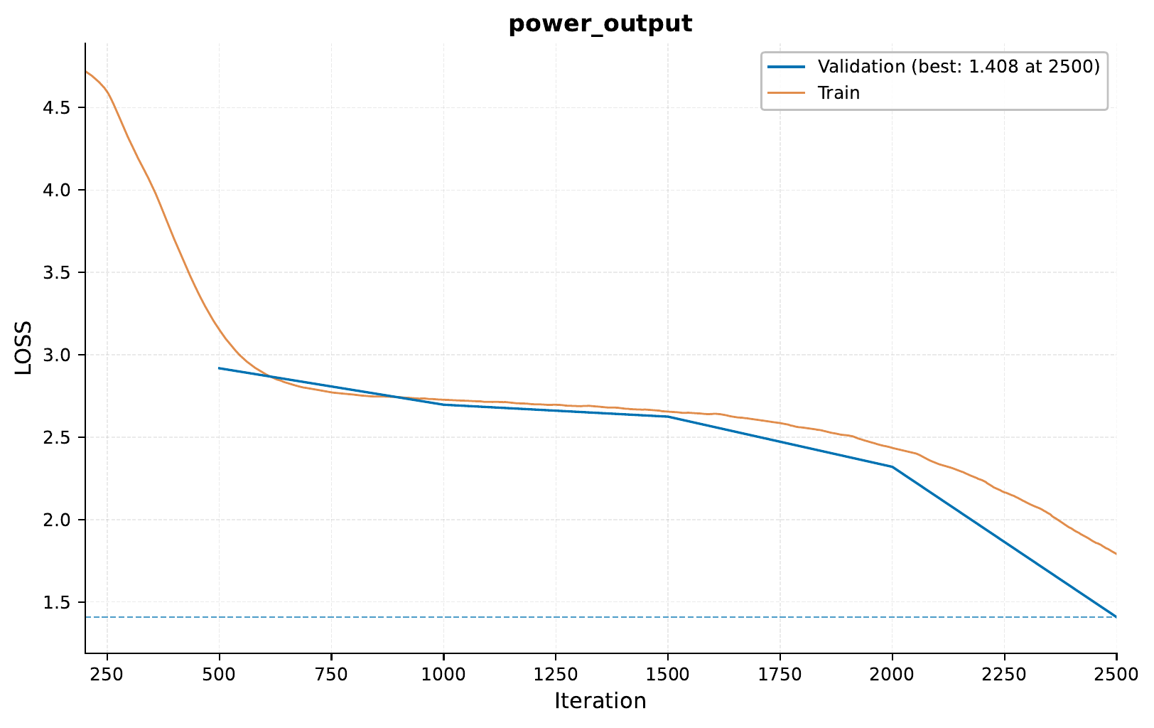
Let’s look at some example predictions:
So, we can see that at least tecnically, the model is able to capture some of the patterns in the simulated data.
Real-World Data Model
For our real-world power consumption prediction task, we use the “Individual Household Electric Power Consumption” dataset from the UCI Machine Learning Repository [1]. This dataset contains measurements of electric power consumption in one household with a one-minute sampling rate over a period of almost 4 years (December 2006 to November 2010).
The dataset above has been processed as follows:
Resampling: - Resampled to 20-minute intervals.
Discretization: - Convert continuous power values into 128 discrete bins.
Data Splitting: - Divide into training and validation (14 days), and test (last 2 weeks) sets. - Splits are made based on non-overlapping sequences.
Sequence Generation: - Create input-output pairs, each spanning 16 hours (48 time steps). - Each pair is based on a sliding window of 1 time step, meaning there is an overlap between samples within each set.
Formatting: - Convert sequences to space-separated integers for model input.
Here are the key configuration files:
basic_experiment:
  batch_size: 64
  memory_dataset: true
  n_epochs: 40
  output_folder: eir_tutorials/tutorial_runs/g_time_series/01_time_series_power_transformer_real
  manual_valid_ids_file: eir_tutorials/g_time_series/01_time_series_power/data/valid_ids.txt
evaluation_checkpoint:
  checkpoint_interval: 100
  n_saved_models: 1
  sample_interval: 100
optimization:
  lr: 0.001
  optimizer: adabelief
input_info:
  input_source: eir_tutorials/g_time_series/01_time_series_power/data/real_input_sequences.csv
  input_name: power_input
  input_type: sequence

input_type_info:
  max_length: 48
  split_on: " "
  sampling_strategy_if_longer: "from_start"
  min_freq: 1

model_config:
  embedding_dim: 64
  model_init_config:
    num_layers: 4
output_info:
  output_source: eir_tutorials/g_time_series/01_time_series_power/data/real_output_sequences.csv
  output_name: power_output
  output_type: sequence

output_type_info:
  max_length: 48
  split_on: " "
  sampling_strategy_if_longer: "from_start"
  min_freq: 1

model_config:
  embedding_dim: 64
  model_init_config:
    num_layers: 4

sampling_config:
  generated_sequence_length: 64
  n_eval_inputs: 10
To train the model on real-world data, run:
eirtrain \
--global_configs eir_tutorials/g_time_series/01_time_series_power/conf/globals_real.yaml \
--fusion_configs eir_tutorials/g_time_series/01_time_series_power/conf/fusion.yaml \
--input_configs eir_tutorials/g_time_series/01_time_series_power/conf/input_sequence_real.yaml \
--output_configs eir_tutorials/g_time_series/01_time_series_power/conf/output_real.yaml
Results and Visualization (Real-World Data)
Here’s the training curve for our real-world data model:

So we can see here that the model starts to overfit relatively early on the training data. This is likely due to the limited amount of effectively unique data after our preprocessing steps.
You may notice some overfitting in our real-life model, as evidenced by the divergence between training and validation loss curves. This is likely due to the limited amount of effectively unique data after our preprocessing steps. After resampling to 20-minute intervals and creating sequences of length 48 (16 hours), we end up with approximately 2,000 non-overlapping samples, even though in our training data we have 100k samples (due to the sliding window approach).
Example predictions on the validation set:
C - Serving
In this final section, we’ll serve our trained model for power consumption prediction as a web service and interact with it using HTTP requests.
Starting the Web Service
To serve the model, use the following command:
eirserve \
--model-path eir_tutorials/tutorial_runs/g_time_series/01_time_series_power_transformer_real/saved_models/01_time_series_power_transformer_real_checkpoint_1800_perf-average=-1.8878.pt
Sending Requests
With the server running, we can now send requests with power consumption data.
Python Example:
import requests


def send_request(url: str, payload: list[dict]) -> list[dict]:
    response = requests.post(url, json=payload)
    response.raise_for_status()
    return response.json()


payload = [
    {
        "power_input": "19 3 10 11 14 3 3 4 4 9 39 27 12 5 20 20 38 39 41 61 "
        "52 31 43 31",
        "power_output": "",
    },
]

response = send_request(url="http://localhost:8000/predict", payload=payload)
print(response)
Bash Example:
curl -X POST \
"http://localhost:8000/predict" \
-H "accept: application/json" \
-H "Content-Type: application/json" \
-d '[{
    "power_input": "19 3 10 11 14 3 3 4 4 9 39 27 12 5 20 20 38 39 41 61 52 31 43 31",
    "power_output": ""
}]'
Analyzing Responses
Now we can play a bit with the served model and see how it responds to our requests. Below are 5 unique requests, but each one of them is repeated 5 times to show the model’s consistency. It would probably be better to use 3 unique models to get a better estimate of the uncertainty, but we will make do with 1 for now.
After sending requests to the served model, let’s analyze the responses:
[
    {
        "request": [
            {
                "power_input": "5 4 2 4 2 4 3 4 20 19 3 2 4 2 4 2 3 4 4 4 10 40 42 39 31 33 21 22 22 22 26 20 23 22 21 13 4 4 3 5 4 4 4 3 3 2 4 2",
                "power_output": ""
            },
            {
                "power_input": "5 4 2 4 2 4 3 4 20 19 3 2 4 2 4 2 3 4 4 4 10 40 42 39 31 33 21 22 22 22 26 20 23 22 21 13 4 4 3 5 4 4 4 3 3 2 4 2",
                "power_output": ""
            },
            {
                "power_input": "5 4 2 4 2 4 3 4 20 19 3 2 4 2 4 2 3 4 4 4 10 40 42 39 31 33 21 22 22 22 26 20 23 22 21 13 4 4 3 5 4 4 4 3 3 2 4 2",
                "power_output": ""
            },
            {
                "power_input": "5 4 2 4 2 4 3 4 20 19 3 2 4 2 4 2 3 4 4 4 10 40 42 39 31 33 21 22 22 22 26 20 23 22 21 13 4 4 3 5 4 4 4 3 3 2 4 2",
                "power_output": ""
            },
            {
                "power_input": "5 4 2 4 2 4 3 4 20 19 3 2 4 2 4 2 3 4 4 4 10 40 42 39 31 33 21 22 22 22 26 20 23 22 21 13 4 4 3 5 4 4 4 3 3 2 4 2",
                "power_output": ""
            },
            {
                "power_input": "2 4 2 4 4 5 4 14 21 6 4 3 4 32 38 36 52 24 21 19 20 19 20 20 22 20 20 20 21 22 22 23 22 2 3 2 3 2 3 2 11 11 12 10 12 15 17 20",
                "power_output": ""
            },
            {
                "power_input": "2 4 2 4 4 5 4 14 21 6 4 3 4 32 38 36 52 24 21 19 20 19 20 20 22 20 20 20 21 22 22 23 22 2 3 2 3 2 3 2 11 11 12 10 12 15 17 20",
                "power_output": ""
            },
            {
                "power_input": "2 4 2 4 4 5 4 14 21 6 4 3 4 32 38 36 52 24 21 19 20 19 20 20 22 20 20 20 21 22 22 23 22 2 3 2 3 2 3 2 11 11 12 10 12 15 17 20",
                "power_output": ""
            },
            {
                "power_input": "2 4 2 4 4 5 4 14 21 6 4 3 4 32 38 36 52 24 21 19 20 19 20 20 22 20 20 20 21 22 22 23 22 2 3 2 3 2 3 2 11 11 12 10 12 15 17 20",
                "power_output": ""
            },
            {
                "power_input": "2 4 2 4 4 5 4 14 21 6 4 3 4 32 38 36 52 24 21 19 20 19 20 20 22 20 20 20 21 22 22 23 22 2 3 2 3 2 3 2 11 11 12 10 12 15 17 20",
                "power_output": ""
            },
            {
                "power_input": "3 3 11 27 33 36 52 31 28 14 35 10 10 11 10 5 3 20 20 7 5 6 5 3 4 3 3 3 3 4 4 4 7 9 16 24 26 25 29 46 47 39 21 29 22 22 21 21",
                "power_output": ""
            },
            {
                "power_input": "3 3 11 27 33 36 52 31 28 14 35 10 10 11 10 5 3 20 20 7 5 6 5 3 4 3 3 3 3 4 4 4 7 9 16 24 26 25 29 46 47 39 21 29 22 22 21 21",
                "power_output": ""
            },
            {
                "power_input": "3 3 11 27 33 36 52 31 28 14 35 10 10 11 10 5 3 20 20 7 5 6 5 3 4 3 3 3 3 4 4 4 7 9 16 24 26 25 29 46 47 39 21 29 22 22 21 21",
                "power_output": ""
            },
            {
                "power_input": "3 3 11 27 33 36 52 31 28 14 35 10 10 11 10 5 3 20 20 7 5 6 5 3 4 3 3 3 3 4 4 4 7 9 16 24 26 25 29 46 47 39 21 29 22 22 21 21",
                "power_output": ""
            },
            {
                "power_input": "3 3 11 27 33 36 52 31 28 14 35 10 10 11 10 5 3 20 20 7 5 6 5 3 4 3 3 3 3 4 4 4 7 9 16 24 26 25 29 46 47 39 21 29 22 22 21 21",
                "power_output": ""
            }
        ],
        "response": {
            "result": [
                {
                    "power_output": "4 2 3 2 3 3 3 3 5 4 3 4 2 8 7 18 29 23 21 23 20 20 19 20 20 19 21 19 19 20 19 22 19 20 22 21 20 20 20 20 19 6 3 4 4 3 5 4 4 8 5 15 25 27 26 27 23 24 30 25 25 25 26"
                },
                {
                    "power_output": "3 4 2 3 3 4 3 18 24 31 29 25 25 23 20 21 20 19 22 20 20 21 20 20 20 21 21 21 21 20 6 4 5 5 4 3 4 3 4 3 4 3 5 6 4 4 5 4 3 4 3 4 4 11 21 8 4 4 8 20 12 9 9"
                },
                {
                    "power_output": "3 3 3 3 3 4 3 4 3 4 17 21 16 6 4 5 9 11 11 13 8 10 14 22 19 9 5 3 4 3 3 4 3 4 3 3 3 3 3 3 3 3 4 3 4 4 3 4 4 3 18 26 31 38 41 36 34 25 26 25 25 23 25"
                },
                {
                    "power_output": "3 3 3 3 3 3 3 3 3 3 5 21 32 26 30 29 23 20 21 21 20 20 20 21 20 20 20 22 19 20 20 21 21 21 21 21 20 21 21 21 21 21 22 20 20 20 20 21 20 24 20 21 22 20 20 21 21 22 19 20 24 20 22"
                },
                {
                    "power_output": "3 3 3 4 2 3 3 17 21 5 3 3 4 5 7 5 7 9 8 7 9 9 11 9 7 7 7 8 7 8 6 6 6 7 8 9 8 7 7 9 12 12 10 10 10 11 20 25 33 35 31 33 38 26 19 27 29 31 30 25 24 22 20"
                },
                {
                    "power_output": "21 21 22 19 6 5 3 4 3 2 3 3 3 4 3 4 2 3 2 3 3 4 3 3 3 3 2 3 3 5 4 3 3 3 3 4 18 22 11 12 29 28 30 24 20 19 19 21 21 19 20 19 22 19 19 20 21 19 22 23 22 20 21"
                },
                {
                    "power_output": "21 21 20 20 19 22 19 20 22 20 20 20 20 20 21 19 5 3 4 4 3 3 3 3 2 3 2 3 2 4 4 2 3 3 4 3 7 20 9 3 2 4 2 4 2 4 2 4 2 5 4 2 3 6 5 4 3 18 23 20 20 20 20"
                },
                {
                    "power_output": "20 20 19 19 20 20 20 20 21 19 20 20 19 20 21 20 21 19 20 20 19 20 20 22 20 20 19 20 20 19 19 19 19 18 21 20 20 20 19 21 20 21 20 20 20 20 19 20 20 20 20 20 21 20 21 19 19 19 22 20 21 20 21"
                },
                {
                    "power_output": "20 20 19 19 18 19 20 19 19 21 19 19 19 20 19 18 18 19 20 19 19 19 19 21 20 20 19 20 19 20 20 20 20 20 20 19 19 20 19 20 20 20 19 19 20 22 18 18 20 19 19 19 20 20 19 18 20 20 19 21 17 3 2"
                },
                {
                    "power_output": "24 26 27 28 26 24 24 26 22 20 22 20 20 21 20 21 21 20 22 21 21 19 3 4 3 4 4 3 3 2 5 3 3 3 2 4 3 5 4 4 5 12 33 30 34 34 37 33 24 24 23 22 25 24 24 22 24 22 22 24 22 22 23"
                },
                {
                    "power_output": "22 20 20 21 20 20 19 22 19 21 20 20 20 20 23 18 3 4 4 5 5 4 5 3 6 8 9 17 23 30 25 27 33 28 29 25 27 28 24 27 27 27 32 36 24 21 20 24 20 21 20 20 20 20 20 22 21 21 21 20 20 22 21"
                },
                {
                    "power_output": "20 22 19 21 22 19 21 20 20 20 21 20 21 20 21 21 23 21 20 22 20 20 20 21 21 22 23 21 24 23 25 25 20 21 21 22 23 21 21 22 21 22 22 22 20 20 21 20 4 4 3 5 5 5 4 3 3 4 4 3 3 3 3"
                },
                {
                    "power_output": "20 21 21 21 21 20 22 20 21 21 21 21 20 20 21 19 21 21 20 20 20 5 4 4 3 3 3 3 4 4 4 4 3 4 3 3 3 4 3 3 3 4 3 3 3 4 3 4 5 3 3 4 3 3 3 4 4 4 4 3 4 4 5"
                },
                {
                    "power_output": "21 23 24 21 22 21 20 22 20 21 20 20 20 21 20 21 20 22 19 3 3 3 4 5 7 4 4 4 3 3 3 3 4 3 4 3 3 4 3 5 4 3 4 4 3 4 3 4 4 3 4 4 5 4 4 4 3 3 3 3 5 5 4"
                },
                {
                    "power_output": "22 22 20 21 20 21 21 20 20 21 20 20 20 19 20 20 20 22 20 4 3 4 3 3 3 3 3 3 4 4 4 4 4 4 5 3 4 3 4 3 5 4 5 6 3 5 3 4 4 4 3 4 4 3 3 4 5 4 4 4 4 4 3"
                }
            ]
        }
    }
]
Visualizing Predictions with Uncertainty
Our model provides predictions with uncertainty estimates. Let’s visualize these:
Conclusion
In this tutorial, we’ve explored how to use EIR for time series prediction tasks, specifically focusing on power consumption forecasting. We’ve covered:
Working with both simulated and real-world datasets
Configuring and training models for each dataset
Visualizing training progress and model predictions
Serving the trained model as a web service
Interacting with the served model using both Python and Bash
Analyzing and visualizing model predictions, including uncertainty estimates
If you made it this far, thank you for reading! We hope this tutorial was interesting and useful to you!