Survival Analysis: Free Light Chain Analysis

In this tutorial, we will explore using EIR for survival analysis tasks, specifically focusing on predicting survival outcomes based on serum free light chain data. We’ll work with a real-world dataset from a Mayo Clinic study that investigated the relationship between serum free light chain levels and mortality in the general population.

Note

This tutorial assumes you are familiar with the basics of EIR and have gone through previous tutorials. Not required, but recommended.

A - Dataset Overview

We’ll be using the Free Light Chain (FLChain) dataset from the Mayo Clinic study, which contains:

• 7,874 subjects

• 9 features including:

  • age: Age in years

  • sex: Gender (F=female, M=male)

  • kappa: Serum free light chain, kappa portion

  • lambda: Serum free light chain, lambda portion

  • flc.grp: Serum free light chain group

  • creatinine: Serum creatinine

  • mgus: Monoclonal gammopathy diagnosis status

• The endpoint is death, which occurred for 2,169 subjects (27.5%)

Note

The dataset comes from a study investigating how non-clonal serum immunoglobulin free light chains can predict overall survival in the general population. More details can be found in the Mayo Clinic Proceedings paper by Dispenzieri et al. (2012).

To download the data, use this link.

After downloading the data, the folder structure should look like this:

eir_tutorials/h_survival_analysis/01_flchain/
├── conf
│   ├── fusion.yaml
│   ├── globals.yaml
│   ├── input.yaml
│   └── output.yaml
└── data
    ├── column_descriptions.txt
    ├── flchain_test.csv
    ├── flchain_train.csv
    ├── test_ids.txt
    └── train_ids.txt

B - Training a Survival Model

Let’s configure and train a model on the FLChain data. Here are the key configuration files:

globals.yaml

basic_experiment:
  n_epochs: 50
  output_folder: eir_tutorials/tutorial_runs/h_survival_analysis/01_flchain
evaluation_checkpoint:
  checkpoint_interval: 100
  n_saved_models: 1
  sample_interval: 100

input.yaml

input_info:
  input_source: eir_tutorials/h_survival_analysis/01_flchain/data/flchain_train.csv
  input_name: flchain
  input_type: tabular

input_type_info:
  input_cat_columns:
    - flcgrp
    - mgus
    - sex
  input_con_columns:
    - age
    - creatinine
    - kappa
    - lambdaport

model_config:
  model_type: tabular

fusion.yaml

model_type: mlp-residual
model_config:
  rb_do: 0.20
  fc_do: 0.20

output.yaml

output_info:
  output_source: eir_tutorials/h_survival_analysis/01_flchain/data/flchain_train.csv
  output_name: flchain_prediction
  output_type: survival
output_type_info:
  time_columns:
    - time
  event_columns:
    - event

To train the model, run the following command:

eirtrain \
--global_configs eir_tutorials/h_survival_analysis/01_flchain/conf/globals.yaml \
--input_configs eir_tutorials/h_survival_analysis/01_flchain/conf/input.yaml \
--fusion_configs eir_tutorials/h_survival_analysis/01_flchain/conf/fusion.yaml \
--output_configs eir_tutorials/h_survival_analysis/01_flchain/conf/output.yaml

Results and Model Performance

Here’s the training curve showing the C-index (concordance index) over time:

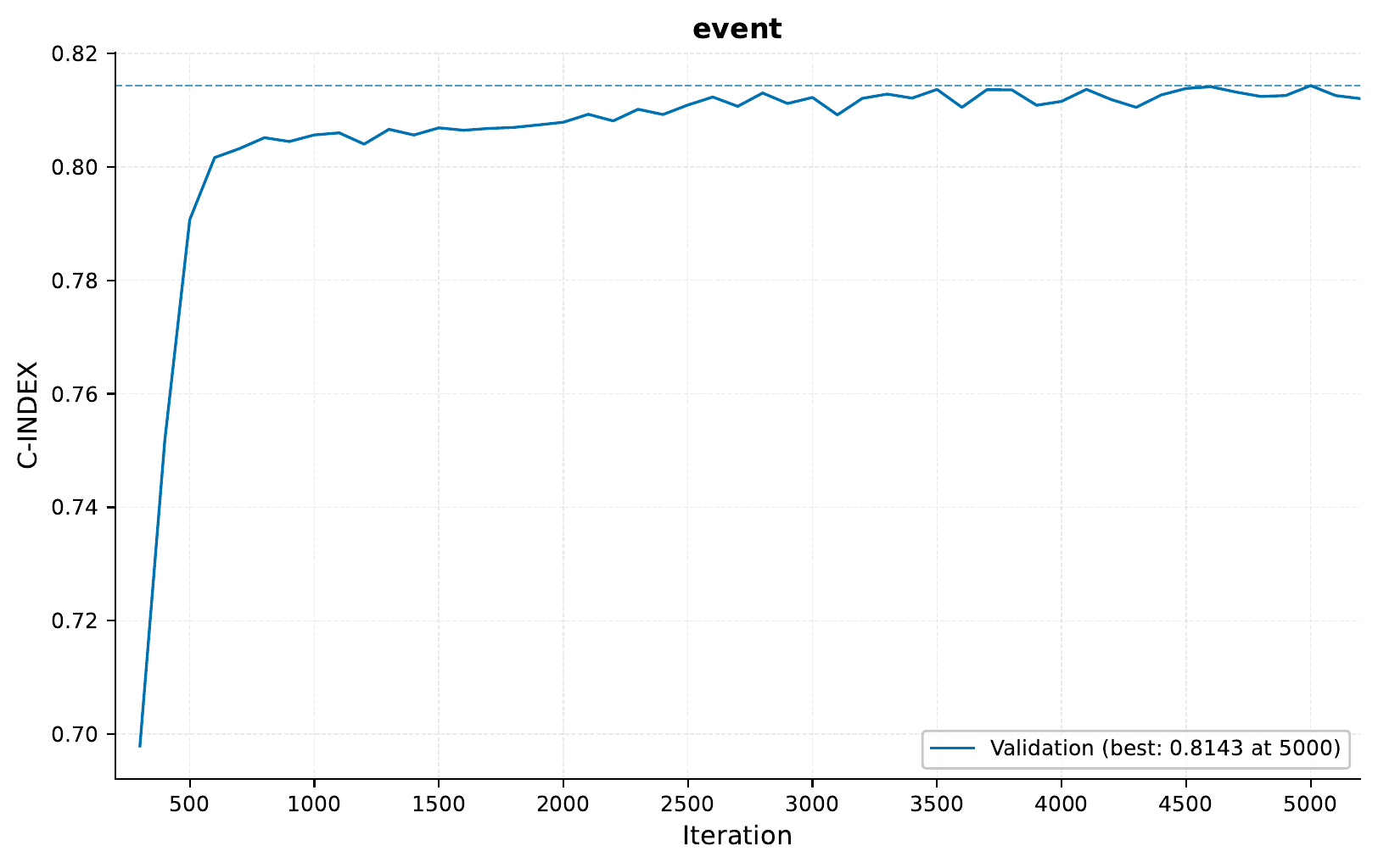
The C-index is a measure of the model’s discrimination ability in survival analysis. A C-index of 0.5 indicates random predictions, while 1.0 indicates perfect discrimination. Our model achieves a C-index of around 0.8 on the validation set, indicating good predictive performance.

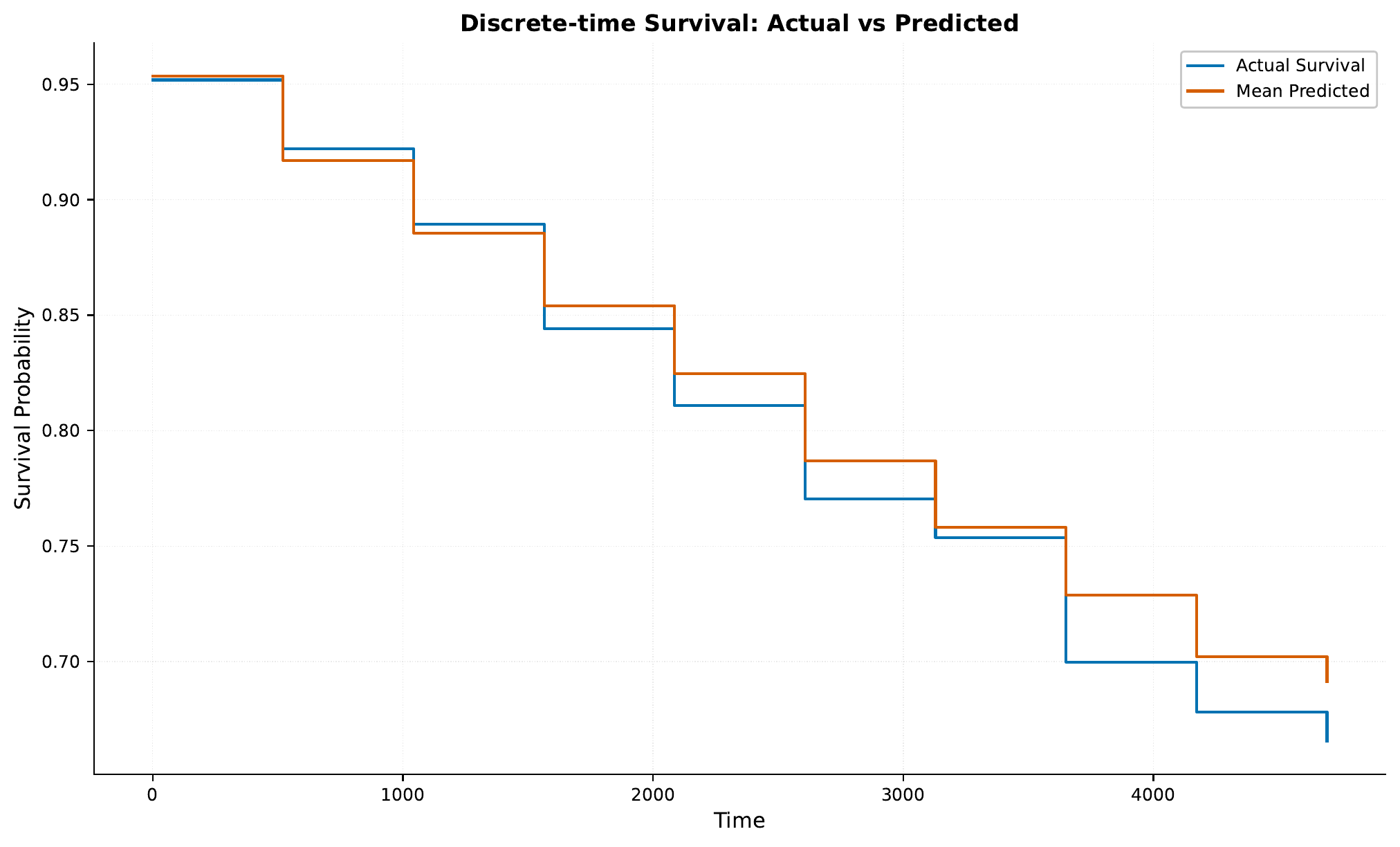
For a given sampling iteration, some survival curves are plotted in the results/samples/<iteration>/ directory.

C - Model Deployment and Analysis

Let’s deploy our trained model as a web service and analyze its predictions across different patient subgroups.

Starting the Web Service

To serve the model, use:

eirserve \
--model-path eir_tutorials/tutorial_runs/h_survival_analysis/01_flchain/saved_models/01_flchain_checkpoint_5000_perf-average=0.8143.pt

Making Predictions

Here’s how to send requests to the model:

Python request example

import requests


def send_request(url: str, payload: list[dict]):
    response = requests.post(url, json=payload)
    return response.json()


payload = [
    {
        "flchain": {
            "age": 65,
            "sex": "M",
            "flcgrp": "1",
            "kappa": 1.5,
            "lambdaport": 1.2,
            "creatinine": 1.1,
            "mgus": "yes",
        }
    }
]

response = send_request(url="http://localhost:8000/predict", payload=payload)
print(response)

Here is an example of the response:

Survival response example

{
    "result": [
        {
            "flchain_prediction": {
                "event": {
                    "time_points": [
                        0.0,
                        521.5,
                        1043.0,
                        1564.5,
                        2086.0,
                        2607.5,
                        3129.0,
                        3650.5,
                        4172.0,
                        4693.5
                    ],
                    "survival_probs": [
                        0.9946708083152771,
                        0.9739656448364258,
                        0.9630329012870789,
                        0.9578489661216736,
                        0.9479295015335083,
                        0.9382162094116211,
                        0.8892793655395508,
                        0.8531079292297363,
                        0.8355057835578918,
                        0.8260446190834045
                    ]
                }
            }
        }
    ]
}

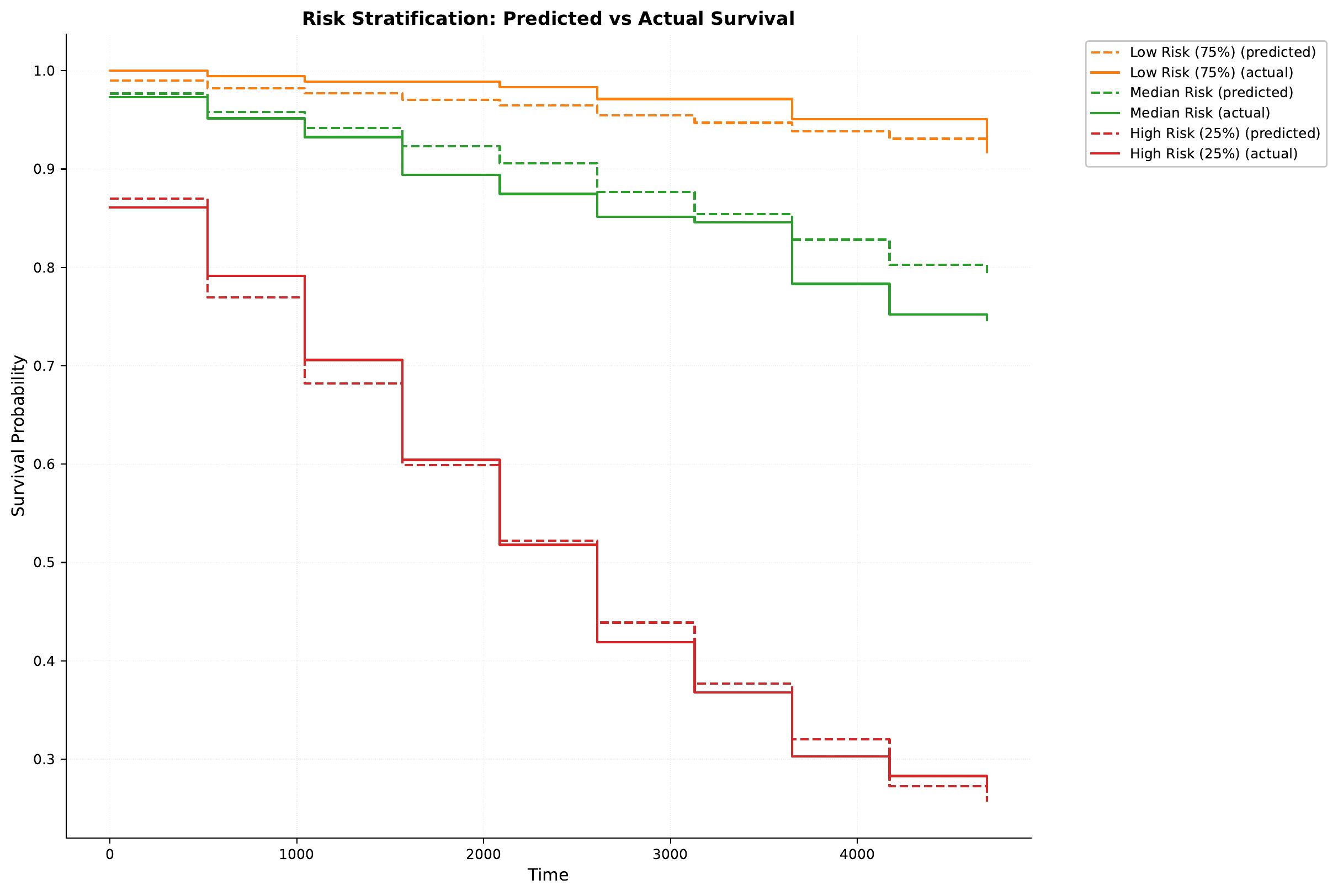
Survival Analysis by Age Groups

After sending all the samples in the test set to the model, we can analyze the survival probabilities across different patient subgroups. Here is how that looks:

Here we can see for example, as expected, that older patients have lower survival probabilities.

Conclusion

In this tutorial, we’ve explored how to:

1. Work with real-world survival analysis data

2. Configure and train a survival prediction model

3. Deploy the model as a web service

4. Analyze survival probabilities across different patient subgroups

If you made it this far, thank you for reading! We hope this tutorial provided useful insights into applying deep learning to survival analysis tasks.