Survival Analysis: Cox Proportional Hazards Model
In this tutorial, we will explore using a Cox Proportional Hazards model for survival analysis with EIR. We’ll use the same Free Light Chain dataset as in the previous tutorial, but this time using a continuous-time approach rather than discrete-time bins.
Note
This tutorial builds on Survival Analysis: Free Light Chain Analysis. Please make sure you’re familiar with that tutorial first, as we’ll be using the same dataset and similar concepts.
A - Dataset Overview
We’ll be using the same Free Light Chain (FLChain) dataset from the Mayo Clinic study as in the previous tutorial. For details about the dataset, please refer to Survival Analysis: Free Light Chain Analysis.
The folder structure should look like this:
eir_tutorials/h_survival_analysis/02_flchain_cox/
├── conf
│   ├── fusion.yaml
│   ├── globals.yaml
│   ├── input.yaml
│   └── output.yaml
└── data
    ├── column_descriptions.txt
    ├── flchain_test.csv
    ├── flchain_train.csv
    ├── test_ids.txt
    └── train_ids.txt
B - Training a Cox Model
Let’s configure and train a Cox model on the FLChain data. The key difference from the previous tutorial is that we’ll use the Cox Proportional Hazards loss function instead of discretizing the time axis. Here are the configuration files:
basic_experiment:
  n_epochs: 50
  output_folder: eir_tutorials/tutorial_runs/h_survival_analysis/02_flchain_cox
evaluation_checkpoint:
  checkpoint_interval: 100
  n_saved_models: 1
  sample_interval: 100
attribution_analysis:
  attributions_every_sample_factor: 4
  compute_attributions: true
  max_attributions_per_class: 512
Notice also here that we are using some flags for attribution analysis, which is also supported for survival models (as well as tabular, i.e. supervised outputs).
input_info:
  input_source: eir_tutorials/h_survival_analysis/01_flchain/data/flchain_train.csv
  input_name: flchain
  input_type: tabular

input_type_info:
  input_cat_columns:
    - flcgrp
    - mgus
    - sex
  input_con_columns:
    - age
    - creatinine
    - kappa
    - lambdaport

model_config:
  model_type: tabular
model_type: mlp-residual
model_config:
  rb_do: 0.20
  fc_do: 0.20
output_info:
  output_source: eir_tutorials/h_survival_analysis/01_flchain/data/flchain_train.csv
  output_name: flchain_prediction
  output_type: survival
output_type_info:
  time_columns:
    - time
  event_columns:
    - event
  loss_function: CoxPHLoss
  num_durations: 0
Note the key difference in output.yaml where we specify “CoxPHLoss” as our loss function.
To train the model, run:
eirtrain \
--global_configs eir_tutorials/h_survival_analysis/02_flchain_cox/conf/globals.yaml \
--input_configs eir_tutorials/h_survival_analysis/02_flchain_cox/conf/input.yaml \
--fusion_configs eir_tutorials/h_survival_analysis/02_flchain_cox/conf/fusion.yaml \
--output_configs eir_tutorials/h_survival_analysis/02_flchain_cox/conf/output.yaml
Results and Model Performance
Here’s the training curve showing the C-index (concordance index) over time:
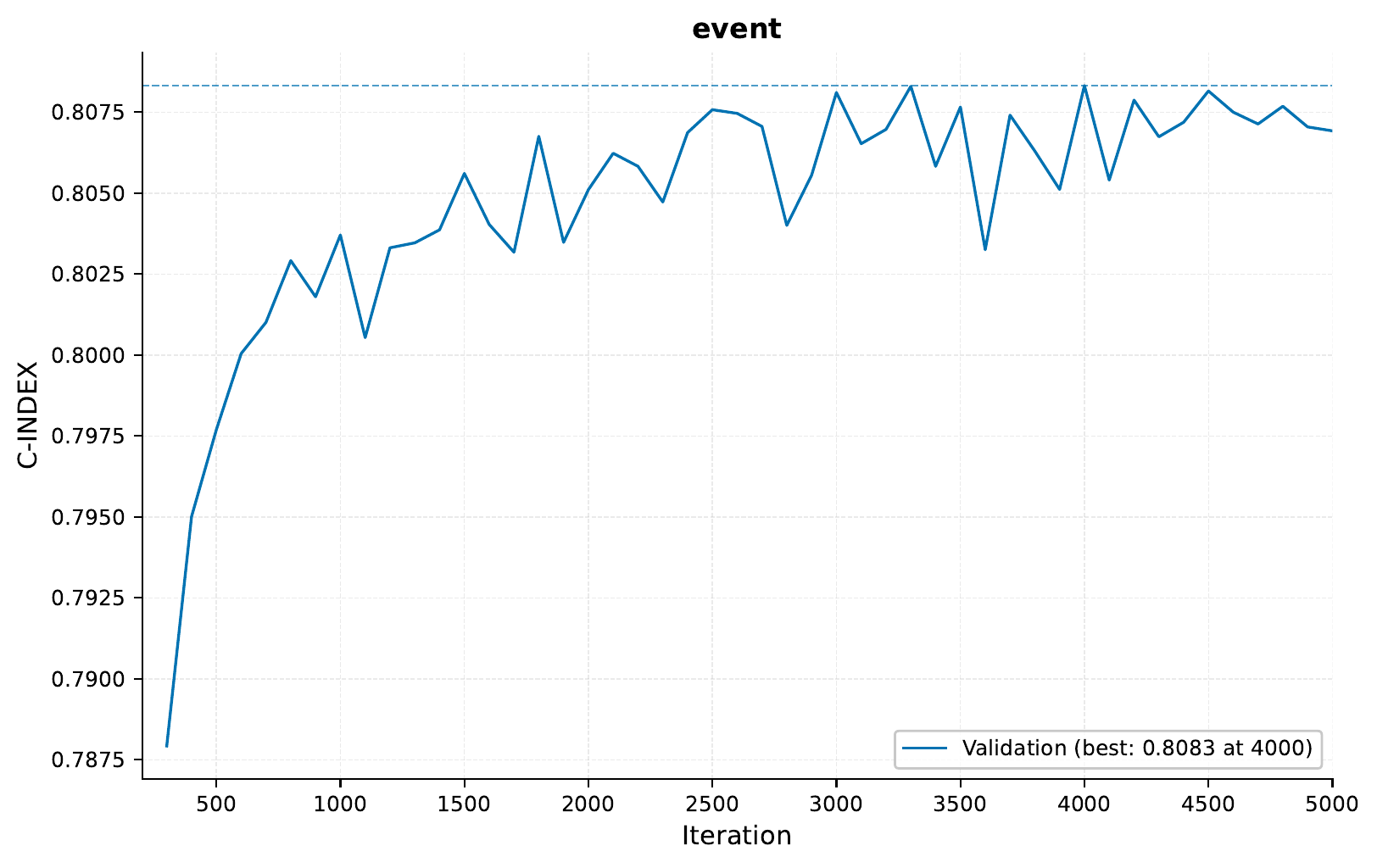
As in the previous tutorial, our model achieves good discrimination with a C-index around 0.8 on the validation set.
The model generates survival curves for visualization. Here are some examples from the
results/samples/<iteration>/ directory:

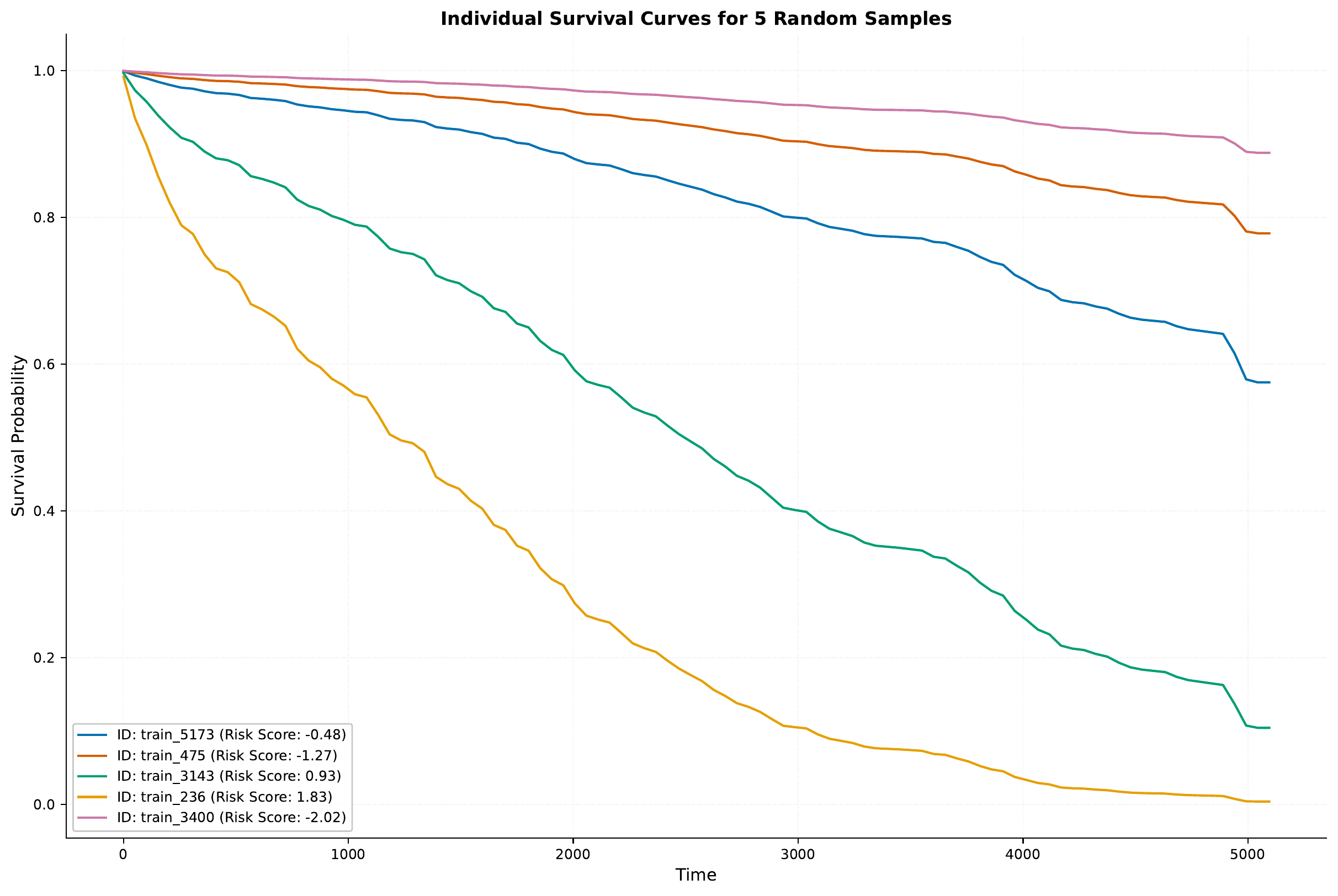
Notice how these curves are smoother than in the discrete-time model, as we’re not restricted to fixed time intervals.
Now, you might remember from above that we set the attribution_analysis flag to True
for the current experiments. If we look under results/samples/<iteration>/attribution/,
we can find various information on how the input features contribute to the model’s predictions
towards a higher risk score.
First, let’s take a look at the overall feature importance:
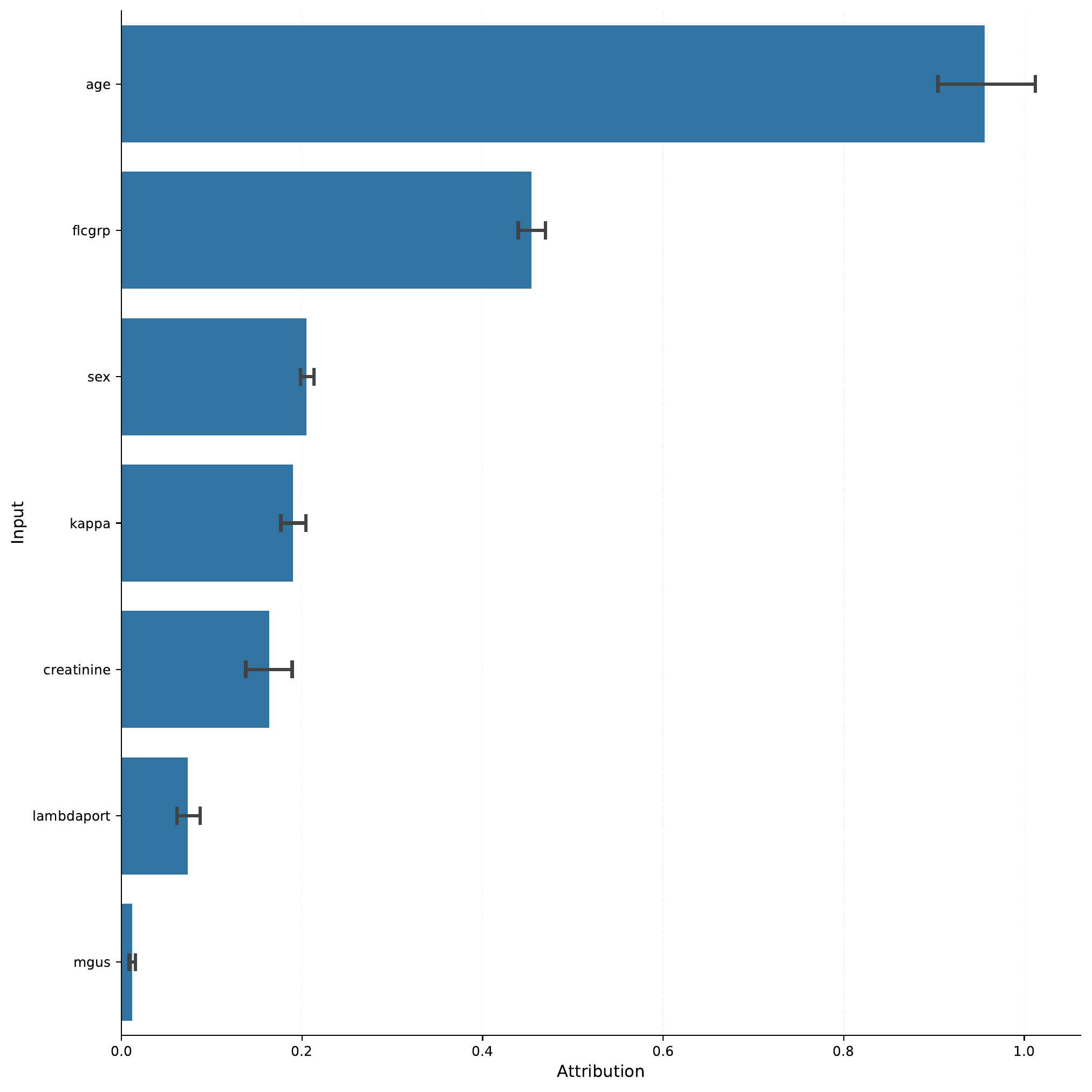
So, perhaps unsurprisingly, the age feature is
the most important feature in the model. We can take a look
at the continuous_attributions.png file to see how the
age feature (and others) contributes to the risk score.

Indeed, with increasing age (here normalized), the risk score increases.
We can also take a look at the feature importance of categorical inputs, here the sex feature:
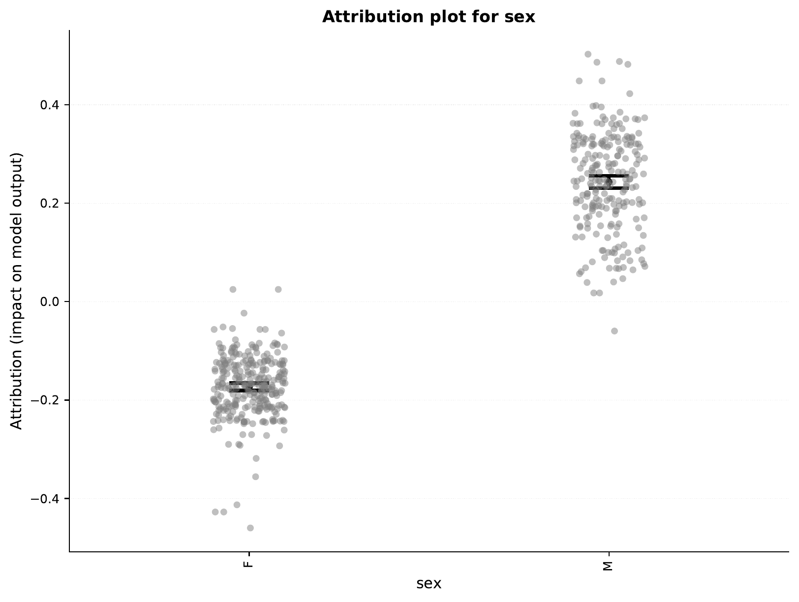
So, the model seems to assign higher risk to males compared to females.
C - Model Deployment and Analysis
Let’s deploy and analyze our Cox model.
Starting the Web Service
To serve the model:
eirserve \
--model-path eir_tutorials/tutorial_runs/h_survival_analysis/02_flchain_cox/saved_models/02_flchain_cox_checkpoint_4000_perf-average=0.8083.pt
Making Predictions
Here’s an example of sending requests to the model:
import requests


def send_request(url: str, payload: list[dict]):
    response = requests.post(url, json=payload)
    return response.json()


payload = [
    {
        "flchain": {
            "age": 65,
            "sex": "M",
            "flcgrp": "1",
            "kappa": 1.5,
            "lambdaport": 1.2,
            "creatinine": 1.1,
            "mgus": "yes",
        }
    }
]

response = send_request(url="http://localhost:8000/predict", payload=payload)
print(response)
Note that unlike the discrete-time model, this model returns risk scores that are then converted to survival probabilities using the baseline hazard function.
Here is an example of the response:
{
"result": [
{
"flchain_prediction": {
"event": {
"survival_probs": [
[
0.9995298389810653,
0.9963576244538855,
0.9941168111590525,
0.9914742757868725,
0.9889919437827357,
0.9870492742546583,
0.9860906674200476,
0.9841237101996906,
0.9826358686253064,
0.9822530946478186,
0.9812817410969128,
0.9795347618596204,
0.9782515786913185,
0.9775870130950943,
0.976555914367657,
0.9740609214665881,
0.9723830415258128,
0.9716289728950548,
0.9702309990318398,
0.9693310082761294,
0.968029484708904,
0.9676218818297778,
0.9657730428631345,
0.9642955155394516,
0.9615592475468301,
0.9611694095330156,
0.9601871712694726,
0.958026906131788,
0.9547492004788665,
0.9542098434489847,
0.9524803570061396,
0.9513746585458781,
0.9486959261886652,
0.9467604834190241,
0.9456908820149394,
0.9425643670110502,
0.9403003430457085,
0.9376122088838217,
0.9353399906763517,
0.9314027072747663,
0.9292002355548538,
0.9259551788872155,
0.9249716762040204,
0.9241325304901055,
0.9201079804769132,
0.917766189877727,
0.9161765949456153,
0.9150060741367626,
0.9118219013224503,
0.9088245779720896,
0.9065713583394899,
0.9040161885862167,
0.9002734360057317,
0.8975149410671406,
0.8940200870326644,
0.892349877865477,
0.88958830272099,
0.8859225518793157,
0.8814122342651711,
0.8804689540621335,
0.8796940263378963,
0.8757955955856276,
0.872784109797244,
0.8710614289024969,
0.8694354870765331,
0.8668095539252583,
0.8647804662456259,
0.8643103192245032,
0.8638397894520333,
0.8632640887110165,
0.8626129097369752,
0.8598192684672337,
0.8589508280364239,
0.8570016731473975,
0.8527877305426573,
0.8480987588250171,
0.8431922570381863,
0.8406963973644781,
0.8345813108955408,
0.8294978651013174,
0.8205633309098073,
0.8179115317192154,
0.8131811907457032,
0.8069793070518445,
0.8057292353364763,
0.8041920556640799,
0.8014315791029971,
0.799666993733477,
0.7950028863914993,
0.7914921595114776,
0.7898667077176023,
0.7888955829018667,
0.787922667081091,
0.7831420976165792,
0.7809513142027098,
0.7795310644322051,
0.7781069345208086,
0.7752481590647543,
0.753297045911575,
0.7258626241491698
]
],
"time_points": [
0.0,
50.48484802246094,
100.96969604492188,
151.4545440673828,
201.93939208984375,
252.4242401123047,
302.9090881347656,
353.3939208984375,
403.8787841796875,
454.3636474609375,
504.8484802246094,
555.3333129882812,
605.8181762695312,
656.3030395507812,
706.787841796875,
757.272705078125,
807.757568359375,
858.242431640625,
908.727294921875,
959.2120971679688,
1009.6969604492188,
1060.1817626953125,
1110.6666259765625,
1161.1514892578125,
1211.6363525390625,
1262.1212158203125,
1312.6060791015625,
1363.0909423828125,
1413.57568359375,
1464.060546875,
1514.54541015625,
1565.0302734375,
1615.51513671875,
1666.0,
1716.48486328125,
1766.9697265625,
1817.45458984375,
1867.9393310546875,
1918.4241943359375,
1968.9090576171875,
2019.3939208984375,
2069.878662109375,
2120.363525390625,
2170.848388671875,
2221.333251953125,
2271.818115234375,
2322.302978515625,
2372.787841796875,
2423.272705078125,
2473.757568359375,
2524.242431640625,
2574.727294921875,
2625.212158203125,
2675.697021484375,
2726.181884765625,
2776.666748046875,
2827.1513671875,
2877.63623046875,
2928.12109375,
2978.60595703125,
3029.0908203125,
3079.57568359375,
3130.060546875,
3180.54541015625,
3231.0302734375,
3281.51513671875,
3332.0,
3382.48486328125,
3432.9697265625,
3483.45458984375,
3533.939453125,
3584.42431640625,
3634.9091796875,
3685.393798828125,
3735.878662109375,
3786.363525390625,
3836.848388671875,
3887.333251953125,
3937.818115234375,
3988.302978515625,
4038.787841796875,
4089.272705078125,
4139.75732421875,
4190.2421875,
4240.72705078125,
4291.2119140625,
4341.69677734375,
4392.181640625,
4442.66650390625,
4493.1513671875,
4543.63623046875,
4594.12109375,
4644.60595703125,
4695.0908203125,
4745.57568359375,
4796.060546875,
4846.54541015625,
4897.0302734375,
4947.51513671875,
4998.0
]
}
}
}
]
}
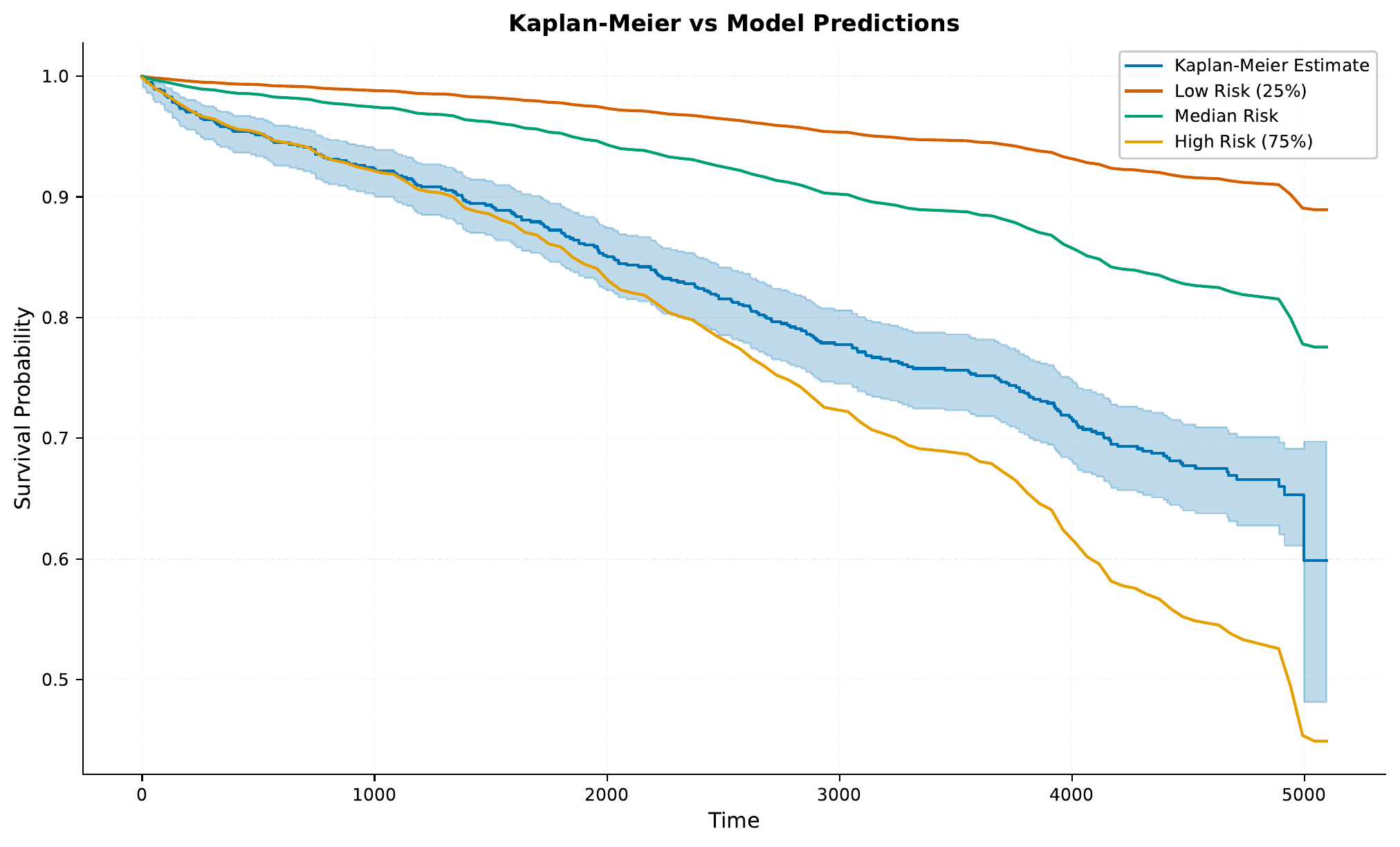
Survival Analysis by Patient Characteristics
After analyzing the test set predictions, here are the survival curves stratified by different patient characteristics:
The smooth curves from the Cox model help visualize the continuous nature of the survival process and the proportional effect of different risk factors.
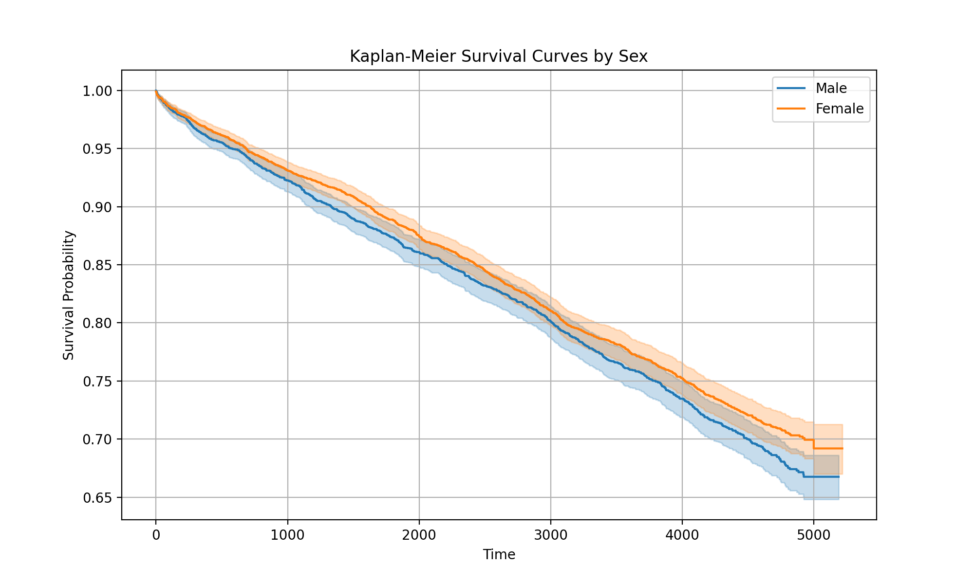
Now, looking at the curve for “sex”, you might notice an interesting discrepancy compared to what we saw earlier with the attributions. The survival seems to have flipped, where now we see higher survival probabilities for males compared females. If we fit and plot a Kaplan-Meier curve for the training data, we see that it does agree with our attributions earlier:
However, when we look at the test data, we see the opposite:
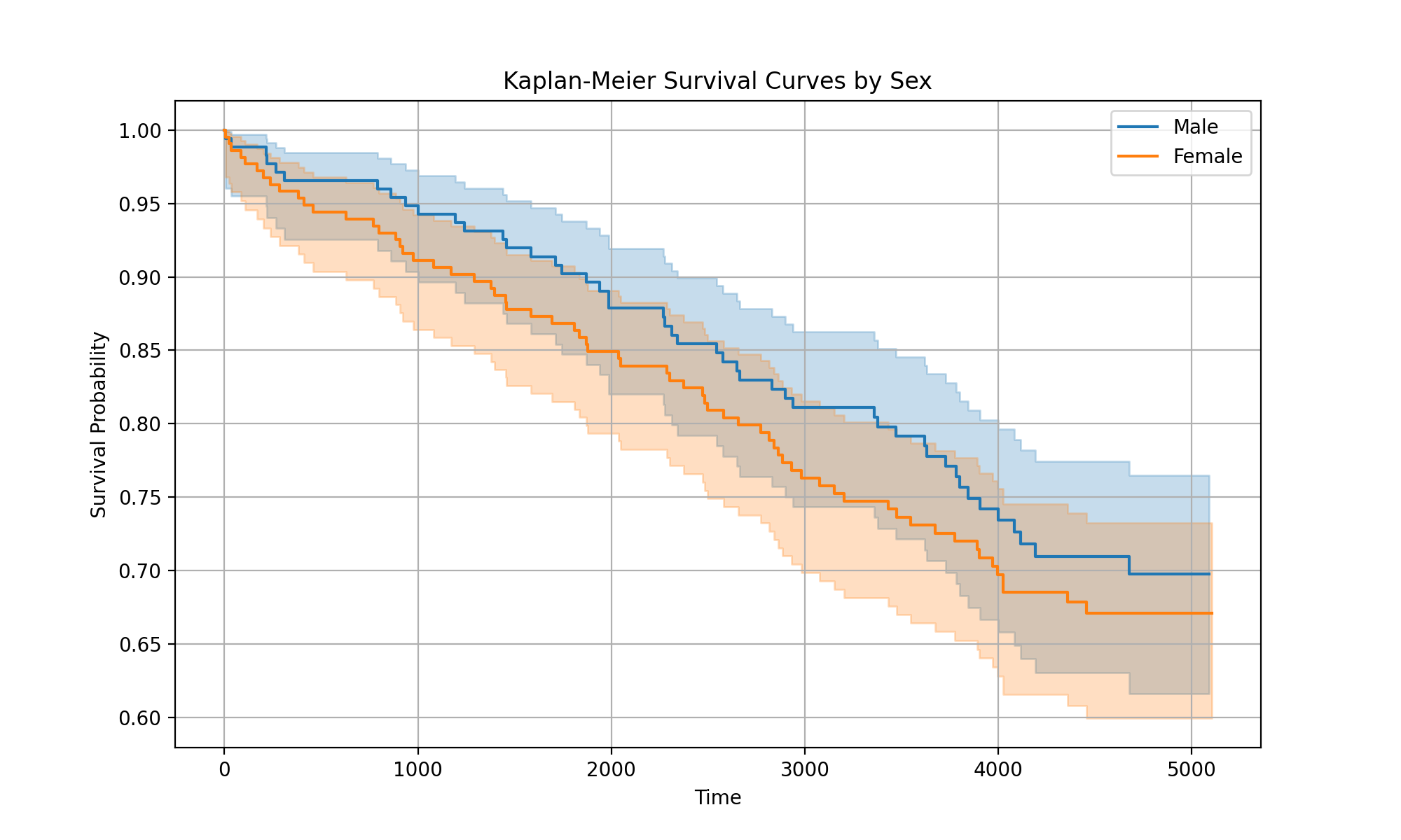
So, it seems that while the model has learned overall that males have higher risk, there might be some other factors in the test data (e.g. due to randomness) where in this subset, males seemingly have lower risk.
Conclusion
In this tutorial, we’ve shown how to:
Configure and train a Cox Proportional Hazards model
Deploy the model as a web service
Generate and interpret continuous survival curves
Analyze survival patterns across patient subgroups