Genotype Tutorial: Ancestry Prediction
A - Setup
In this tutorial, we will be using genotype data to train deep learning models for ancestry prediction.
Note
This tutorial goes into some detail about how EIR works,
and how to use it. If you are more interested in quickly training
the deep learning models for genomic prediction, the EIR-auto-GP
project might be of use to you.
To start, please download processed sample data (or process your own .bed, .bim, .fam files with e.g. plink pipelines). The sample data we are using here for predicting ancestry is the public Human Origins dataset, but the same approach can just as well be used for e.g. disease predictions in other cohorts (for example the UK Biobank).
Examining the sample data, we can see the following structure:
processed_sample_data
├── arrays                      # Genotype data as NumPy arrays
├── data_final_gen.bim          # Variant information file accompanying the genotype arrays
└── human_origins_labels.csv    # Contains the target labels (what we want to predict from the genotype data)
Important
The label file ID column must be called “ID” (uppercase).
For this tutorial, we are going to use the data above to models to predict ancestry, of which there are 6 classes (Asia, Eastern Asia, Europe, Latin America and the Caribbean, Middle East and Sub-Saharan Africa). Before diving into the model training, we first have to configure our experiments.
To configure the experiments we want to run,
we will use .yaml configurations.
Running eirtrain --help,
we can see the configurations needed:
usage: eirtrain [-h] --global_configs GLOBAL_CONFIGS [GLOBAL_CONFIGS ...]
                [--input_configs [INPUT_CONFIGS ...]]
                [--fusion_configs [FUSION_CONFIGS ...]]
                --output_configs OUTPUT_CONFIGS [OUTPUT_CONFIGS ...]

options:
  -h, --help            show this help message and exit
  --global_configs GLOBAL_CONFIGS [GLOBAL_CONFIGS ...]
                        Global .yaml configurations for the experiment.
  --input_configs [INPUT_CONFIGS ...]
                        Input feature extraction .yaml configurations. Each
                        configuration represents one input.
  --fusion_configs [FUSION_CONFIGS ...]
                        Fusion .yaml configurations.
  --output_configs OUTPUT_CONFIGS [OUTPUT_CONFIGS ...]
                        Output .yaml configurations.
Above we can see that there are four types of configurations we can use: global, inputs, fusion and outputs. To see more details about what should be in these configuration files, we can check the Configuration API Reference reference.
Note
Instead of having to type out the configuration files below manually, you can
download them from the docs/tutorials/tutorial_files/01_basic_tutorial directory
in the project repository
While the global configuration has a lot of options,
the only one we really need to fill in now is
output_folder and evaluation interval (in batch iterations),
so we have the following tutorial_01_globals.yaml file:
basic_experiment:
  output_folder: eir_tutorials/tutorial_runs/a_using_eir/tutorial_01_run
evaluation_checkpoint:
  checkpoint_interval: 200
  sample_interval: 200
We also need to tell the framework where to load inputs from,
and some information about the input, for that we use an input .yaml configuration
called tutorial_01_inputs.yaml:
input_info:
  input_source: eir_tutorials/a_using_eir/01_basic_tutorial/data/processed_sample_data/arrays
  input_name: genotype
  input_type: omics

input_type_info:
  snp_file: eir_tutorials/a_using_eir/01_basic_tutorial/data/processed_sample_data/data_final_gen.bim

model_config:
  model_type: genome-local-net
Above we can see that the input needs 3 fields: input_info, input_type_info and
model_config.
The input_info contains basic information about the input.
The input_type_info contains information specific to the input type (in this case
omics).
Finally, the model_config contains configuration for
the model that should be
trained with the input data.
For more information about the
configurations, e.g. which parameters are relevant for the chosen models and what they
do, head over to the Configuration API Reference reference.
Finally, we need to specify what outputs to predict during training. For that we
will use the tutorial_01_outputs.yaml file with the following content:
output_info:
  output_name: ancestry_output
  output_source: eir_tutorials/a_using_eir/01_basic_tutorial/data/processed_sample_data/human_origins_labels.csv
  output_type: tabular
output_type_info:
  target_cat_columns:
    - Origin
Note
You might notice that we have not written any fusion config so far. The fusion configuration controls how different modalities (i.e. input data types, for example genotype and clinical data) are combined using a neural network. While we indeed can configure the fusion, we will leave use the defaults for now. The default fusion model is a fully connected neural network.
With all this, we should have our project directory looking something like this:
eir_tutorials/a_using_eir/01_basic_tutorial/
├── conf
│   ├── tutorial_01_globals.yaml
│   ├── tutorial_01_input.yaml
│   ├── tutorial_01_outputs_unknown.yaml
│   └── tutorial_01_outputs.yaml
└── data
    ├── processed_sample_data
    │   ├── arrays
    │   ├── data_final_gen.bim
    │   └── human_origins_labels.csv
    └── processed_sample_data.zip
B - Training
Training a GLN model
Now that we have our configurations set up, training is simply passing them to the framework, like so:
eirtrain \
--global_configs eir_tutorials/a_using_eir/01_basic_tutorial/conf/tutorial_01_globals.yaml \
--input_configs eir_tutorials/a_using_eir/01_basic_tutorial/conf/tutorial_01_input.yaml \
--output_configs eir_tutorials/a_using_eir/01_basic_tutorial/conf/tutorial_01_outputs.yaml
This will generate a folder in the current directory called eir_tutorials,
and eir_tutorials/tutorial_runs/a_using_eir/tutorial_01_run
(note that the inner run name comes from the value in
global_config we set before)
will contain the results from our experiment.
Tip
You might try running the command above again after it partially/completely
finishes, and most likely you will encounter a FileExistsError.
This is to avoid accidentally overwriting previous experiments. When performing
another run, we will have to delete/rename the experiment, or change it in the
configuration (see below).
Examining the directory, we see the following structure (some files have been excluded here for brevity):
eir_tutorials/tutorial_runs/a_using_eir/tutorial_01_run/
├── configs
├── meta
│   └── eir_version.txt
├── model_info.txt
├── results
│   └── ancestry_output
│       └── Origin
│           ├── samples
│           │   ├── 200
│           │   │   ├── confusion_matrix.pdf
│           │   │   ├── mc_pr_curve.pdf
│           │   │   ├── mc_roc_curve.pdf
│           │   │   └── predictions.csv
│           │   ├── 400
│           │   │   ├── confusion_matrix.pdf
│           │   │   ├── mc_pr_curve.pdf
│           │   │   ├── mc_roc_curve.pdf
│           │   │   └── predictions.csv
│           │   └── 600
│           │       ├── confusion_matrix.pdf
│           │       ├── mc_pr_curve.pdf
│           │       ├── mc_roc_curve.pdf
│           │       └── predictions.csv
│           ├── training_curve_ACC.pdf
│           ├── training_curve_AP-MACRO.pdf
│           ├── training_curve_LOSS.pdf
│           ├── training_curve_MCC.pdf
│           └── training_curve_ROC-AUC-MACRO.pdf
├── saved_models
├── test_predictions
│   ├── known_outputs
│   │   ├── ancestry_output
│   │   │   └── Origin
│   │   │       ├── confusion_matrix.pdf
│   │   │       ├── mc_pr_curve.pdf
│   │   │       ├── mc_roc_curve.pdf
│   │   │       └── predictions.csv
│   │   └── calculated_metrics.json
│   └── unknown_outputs
│       └── ancestry_output
│           └── Origin
│               └── predictions.csv
├── training_curve_LOSS-AVERAGE.pdf
└── training_curve_PERF-AVERAGE.pdf
In the results folder for a given output,
the [200, 400, 600] folders
contain our validation results
according to our sample_interval configuration
in the global config.
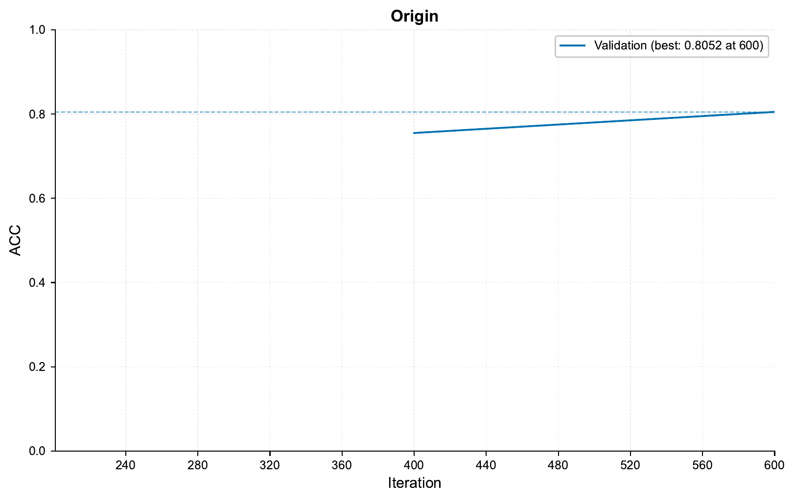
We can examine how our model did with respect to accuracy (let’s assume our targets are fairly balanced in this case) by checking the training_curve_ACC.png file:
Examining the actual predictions and how they matched the target labels,
we can look at the confusion matrix in one of the evaluation folders of
results/Origin/samples. When I ran this, I got the following at iteration 600:

In the training curve above,
we can see that our model barely got going before the run finished!
Let’s try another experiment.
We can change the output_folder value
in 01_basic_tutorial/tutorial_01_globals.yaml,
but the framework also supports rudimentary injection of values from the command line.
Let’s try that,
setting a new run name,
increasing the number of epochs and
changing the learning rate:
eirtrain \
--global_configs eir_tutorials/a_using_eir/01_basic_tutorial/conf/tutorial_01_globals.yaml \
--input_configs eir_tutorials/a_using_eir/01_basic_tutorial/conf/tutorial_01_input.yaml \
--output_configs eir_tutorials/a_using_eir/01_basic_tutorial/conf/tutorial_01_outputs.yaml \
--tutorial_01_globals.basic_experiment.output_folder=eir_tutorials/tutorial_runs/a_using_eir/tutorial_01_run_lr-0.002_epochs-20 \
--tutorial_01_globals.optimization.lr=0.002 \
--tutorial_01_globals.basic_experiment.n_epochs=20
Note
The injected values are according to the configuration filenames.
Looking at the training curve from that run, we can see we did a bit better:

We also notice that there is a gap between the training and evaluation performances, indicating that the model is starting to overfit on the training data. There are a bunch of regularisation settings we could try, such as increasing dropout in the input, fusion and output modules. Check the Configuration API Reference reference for a full overview.
C - Predicting on external samples
Predicting on samples with known labels
To predict on external samples, we run eirpredict.
As we can see when running eirpredict --help, it looks quite
similar to eirtrain:
usage: eirpredict [-h] [--global_configs [GLOBAL_CONFIGS ...]]
                  [--input_configs [INPUT_CONFIGS ...]]
                  [--fusion_configs [FUSION_CONFIGS ...]]
                  [--output_configs [OUTPUT_CONFIGS ...]]
                  --model_path MODEL_PATH [--evaluate]
                  --output_folder OUTPUT_FOLDER
                  [--attribution_background_source {train,predict}]

options:
  -h, --help            show this help message and exit
  --global_configs [GLOBAL_CONFIGS ...]
                        Global .yaml configurations for the experiment.
  --input_configs [INPUT_CONFIGS ...]
                        Input feature extraction .yaml configurations. Each
                        configuration represents one input.
  --fusion_configs [FUSION_CONFIGS ...]
                        Fusion .yaml configurations.
  --output_configs [OUTPUT_CONFIGS ...]
                        Output .yaml configurations.
  --model_path MODEL_PATH
                        Path to model to use for predictions.
  --evaluate
  --output_folder OUTPUT_FOLDER
                        Where to save prediction results.
  --attribution_background_source {train,predict}
                        For attribution analysis, whether to load backgrounds
                        from the data used for training or to use the current
                        data passed to the predict module.
Generally we do not change much of the configs when predicting, with the exception of
the input configs (and then mainly setting the input_source,
i.e. where to load our samples to predict/test on from) and perhaps the global config
(e.g. we might not compute attributions during training, but compute them on our test set
by activating compute_attributions in the global config when predicting). Specific to
eirpredict, we have to choose a saved model (--model_path), whether we want to
evaluate the performance on the test set (--evaluate this means that the respective
labels must be present in the --output_configs) and where to save the prediction
results (--output_folder).
For the sake of this tutorial, we use one of the saved models from our previous training
run and use it for inference using eirpredict module. Here, we will simply use it
to predict on the same data as before.
Warning
We are only predicting on the same data we trained on in this tutorial to show
how to use the eirpredict module. Always take care in separating what data you
use for training and to evaluate generalization performance of your models!
Run the commands below, making sure you add the correct path of a saved model to the
--model_path argument.
To test, we can run the following command
(note that you will have to add the path to your saved model for the --model_path
parameter below).
eirpredict \
--global_configs eir_tutorials/a_using_eir/01_basic_tutorial/conf/tutorial_01_globals.yaml \
--input_configs eir_tutorials/a_using_eir/01_basic_tutorial/conf/tutorial_01_input.yaml \
--output_configs eir_tutorials/a_using_eir/01_basic_tutorial/conf/tutorial_01_outputs.yaml \
--model_path eir_tutorials/tutorial_runs/a_using_eir/tutorial_01_run/saved_models/tutorial_01_run_checkpoint_600_perf-average=0.8573.pt \
--evaluate \
--output_folder eir_tutorials/tutorial_runs/a_using_eir/tutorial_01_run/test_predictions/known_outputs
This will generate a file called
calculated_metrics.json in the supplied output_folder as well
as a folder for each output (in this case called ancestry_output
containing the actual predictions and plots. Of course the metrics are quite nonsensical
here, as we are predicting on the same data we trained on.
One of the files generated are the actual predictions,
found in the predictions.csv file:
| ID | True Label Untransformed |
True Label | Asia | Eastern_Asia | Europe | Latin_America_and_th e_Caribbean |
Middle_East | Sub-Saharan_Africa |
|---|---|---|---|---|---|---|---|---|
| A306 | Europe | 2 | 0.75 | -2.05 | 3.62 | -0.04 | 2.19 | -2.75 |
| A325 | Europe | 2 | 1.50 | -2.84 | 2.49 | -0.18 | 3.26 | -1.64 |
| A343 | Europe | 2 | 0.81 | -2.32 | 2.97 | -0.39 | 3.18 | -1.55 |
| A362 | Europe | 2 | 1.23 | -2.23 | 3.48 | -0.58 | 2.68 | -1.94 |
| A374 | Europe | 2 | 1.46 | -2.39 | 3.10 | -1.72 | 2.98 | -1.46 |
The True Label Untransformed column contains the actual labels, as they were
in the raw data. The True Label column contains the labels after they have been
numerically encoded / normalized in EIR.
The other columns represent the raw network outputs
for each of the classes.
Predicting on samples with unknown labels
Notice that when running the command above, we knew the labels of the samples we were
predicting on. In practice, we are often predicting on samples we have no clue
about the labels of. In this case, we can again use the eirpredict with slightly
modified arguments:
eirpredict \
--global_configs eir_tutorials/a_using_eir/01_basic_tutorial/conf/tutorial_01_globals.yaml \
--input_configs eir_tutorials/a_using_eir/01_basic_tutorial/conf/tutorial_01_input.yaml \
--output_configs eir_tutorials/a_using_eir/01_basic_tutorial/conf/tutorial_01_outputs_unknown.yaml \
--model_path eir_tutorials/tutorial_runs/a_using_eir/tutorial_01_run/saved_models/tutorial_01_run_checkpoint_600_perf-average=0.8573.pt \
--output_folder eir_tutorials/tutorial_runs/a_using_eir/tutorial_01_run/test_predictions/unknown_outputs
We can notice a couple of changes here compared to the previous command:
We have removed the
--evaluateflag, as we do not have the labels for the samples we are predicting on.We have a different output configuation file,
tutorial_01_outputs_unknown.yaml.We have a different output folder,
tutorial_01_unknown.
If we take a look at the tutorial_01_outputs_unknown.yaml file, we can see that
it contains the following:
output_info:
  output_name: ancestry_output
  output_source: null
  output_type: tabular
output_type_info:
  target_cat_columns:
    - Origin
Notice that everything is the same as before, but for output_source we have
null instead of the .csv label file we had before.
Taking a look at the produced predictions.csv file, we can see that we only
have the actual predictions, and no true labels:
| ID | Asia | Eastern_Asia | Europe | Latin_America_and_th e_Caribbean |
Middle_East | Sub-Saharan_Africa |
|---|---|---|---|---|---|---|
| A306 | 0.75 | -2.05 | 3.62 | -0.04 | 2.19 | -2.75 |
| A325 | 1.50 | -2.84 | 2.49 | -0.18 | 3.26 | -1.64 |
| A343 | 0.81 | -2.32 | 2.97 | -0.39 | 3.18 | -1.55 |
| A362 | 1.23 | -2.23 | 3.48 | -0.58 | 2.68 | -1.94 |
| A374 | 1.46 | -2.39 | 3.10 | -1.72 | 2.98 | -1.46 |
D - Serving
In this final section, we demonstrate serving our trained model as a web service and interacting with it using HTTP requests.
Starting the Web Service
To serve the model, use the following command:
eirserve --model-path [MODEL_PATH]
Replace [MODEL_PATH] with the actual path to your trained model. This command initiates a web service that listens for incoming requests.
Here is an example of the command:
eirserve \
--model-path eir_tutorials/tutorial_runs/a_using_eir/tutorial_01_run/saved_models/tutorial_01_run_checkpoint_600_perf-average=0.8573.pt
Note
After serving the model, you can access the automatically generated
OpenAPI documentation at http://localhost:8000/docs to explore and
interact with the API endpoints. Additionally http://localhost:8000/info
provides some basic information about intput/output data specifications.
There is also a UI available at http://localhost:8000/redoc for an
alternative view of the API documentation.
Sending Requests
With the server running, we can now send requests. The requests are prepared by loading numpy array data, converting it to base64 encoded strings, and then constructing a JSON payload.
Here’s an example Python function demonstrating this process:
import base64

import numpy as np
import requests


def encode_numpy_array(file_path: str) -> str:
    array = np.load(file_path)
    encoded = base64.b64encode(array.tobytes()).decode("utf-8")
    return encoded


def send_request(url: str, payload: list[dict]):
    response = requests.post(url, json=payload)
    return response.json()


encoded_data = encode_numpy_array(
    file_path="eir_tutorials/a_using_eir/01_basic_tutorial/data/"
    "processed_sample_data/arrays/A_French-4.DG.npy"
)
response = send_request(
    url="http://localhost:8000/predict", payload=[{"genotype": encoded_data}]
)
print(response)
When running this, we get the following output:
{
    "result": [
        {
            "ancestry_output": {
                "Origin": {
                    "Asia": 0.011007264256477356,
                    "Eastern_Asia": 0.0009965847712010145,
                    "Europe": 0.9667631983757019,
                    "Latin_America_and_the_Caribbean": 0.004406982567161322,
                    "Middle_East": 0.01634623296558857,
                    "Sub-Saharan_Africa": 0.00047989984159357846
                }
            }
        }
    ]
}
Analyzing Responses
Here are some examples of responses from the server for a set of inputs:
[
    {
        "request": [
            {
                "genotype": "eir_tutorials/a_using_eir/01_basic_tutorial/data/processed_sample_data/arrays/A374.npy"
            },
            {
                "genotype": "eir_tutorials/a_using_eir/01_basic_tutorial/data/processed_sample_data/arrays/Ayodo_468C.npy"
            },
            {
                "genotype": "eir_tutorials/a_using_eir/01_basic_tutorial/data/processed_sample_data/arrays/NOR146.npy"
            }
        ],
        "response": {
            "result": [
                {
                    "ancestry_output": {
                        "Origin": {
                            "Asia": 0.09177874028682709,
                            "Eastern_Asia": 0.001957354135811329,
                            "Europe": 0.4765580892562866,
                            "Latin_America_and_the_Caribbean": 0.0038182223215699196,
                            "Middle_East": 0.4209199547767639,
                            "Sub-Saharan_Africa": 0.004967665299773216
                        }
                    }
                },
                {
                    "ancestry_output": {
                        "Origin": {
                            "Asia": 0.004986831918358803,
                            "Eastern_Asia": 0.0022864150814712048,
                            "Europe": 0.008424260653555393,
                            "Latin_America_and_the_Caribbean": 0.046364832669496536,
                            "Middle_East": 0.044497761875391006,
                            "Sub-Saharan_Africa": 0.8934398889541626
                        }
                    }
                },
                {
                    "ancestry_output": {
                        "Origin": {
                            "Asia": 0.024995112791657448,
                            "Eastern_Asia": 0.001728453440591693,
                            "Europe": 0.8829706311225891,
                            "Latin_America_and_the_Caribbean": 0.034079667180776596,
                            "Middle_East": 0.054588526487350464,
                            "Sub-Saharan_Africa": 0.0016375456470996141
                        }
                    }
                }
            ]
        }
    }
]
E - Applying to your own data (e.g. UK Biobank)
Thank you for reading this far! Hopefully this tutorial introduced you well enough to
the framework so you can apply it to your own genetic data.
For that, you will have to process
it first (see: plink pipelines). Then you will have to set the relevant paths for the
inputs (e.g. input_source, snp_file) and outputs
(e.g. output_source, target_cat_columns or target_con_columns
if you have continuous targets).
However, when moving to large scale data such as the UK Biobank, the configurations we used on the ancestry toy data in this tutorial will likely not be sufficient. For example, the learning rate is likely too high. For this, we specifically designed the EIR-auto-GP project, which focuses on allow you to quickly train deep learning models for genomic prediction. Additionally, you can have a look at the Genomics Guide for some more information on the parameters that are relevant for genomic data and how do adapt the configurations to your own data.
If you made it this far, thank you for reading!