Tabular Tutorial: Nonlinear Poker Hands
A - Setup
In this tutorial, we will be training a model using only tabular data as input. The task is to predict poker hands from the suit an rank of cards. See here for more information about the dataset.
Note that this tutorial assumes that you are already familiar with the basic functionality of the framework (see Genotype Tutorial: Ancestry Prediction).
To download the data for for this tutorial, use this link.
Having a quick look at the data, we can see it consists of 10 categorical inputs columns and 1 categorical output column (which has 10 classes).
$ head -n 3 poker_hands_data/poker_hands_train.csv

ID,S1,C1,S2,C2,S3,C3,S4,C4,S5,C5,CLASS
0,2,11,2,13,2,10,2,12,2,1,9
1,3,12,3,11,3,13,3,10,3,1,9
To start with, we can use the following configurations for the global, input, target and predictor parts respectively:
basic_experiment:
  manual_valid_ids_file: eir_tutorials/a_using_eir/02_tabular_tutorial/data/poker_hands_data/pre_split_valid_ids.txt
  n_epochs: 50
  output_folder: eir_tutorials/tutorial_runs/a_using_eir/tutorial_02_run
evaluation_checkpoint:
  checkpoint_interval: 1000
  n_saved_models: 1
  sample_interval: 1000
Note
You might notice the perhaps new manual_valid_ids_file argument
in the global configuration. This is because
the data is quite imbalanced, so we provide a pre-computed validation set to
ensure that all classes are present in both the training and validation set.
Be aware that currently the framework does not handle having a mismatch in which
classes are present in the training and validation sets.
input_info:
  input_source: eir_tutorials/a_using_eir/02_tabular_tutorial/data/poker_hands_data/poker_hands_train.csv
  input_name: poker_hands
  input_type: tabular

input_type_info:
  input_cat_columns:
          - S1
          - C1
          - S2
          - C2
          - S3
          - C3
          - S4
          - C4
          - S5
          - C5

model_config:
  model_type: tabular
model_type: mlp-residual
model_config:
  rb_do: 0.20
  fc_do: 0.20
output_info:
  output_source: eir_tutorials/a_using_eir/02_tabular_tutorial/data/poker_hands_data/poker_hands_train.csv
  output_name: poker_prediction
  output_type: tabular
output_type_info:
  target_cat_columns:
    - CLASS
So, after setting up, our folder structure should look something like this:
eir_tutorials/a_using_eir/02_tabular_tutorial/
├── conf
│   ├── 02_poker_hands_fusion.yaml
│   ├── 02_poker_hands_globals.yaml
│   ├── 02_poker_hands_input.yaml
│   └── 02_poker_hands_output.yaml
└── data
    └── poker_hands_data
        ├── poker_hands_test.csv
        ├── poker_hands_train.csv
        └── pre_split_valid_ids.txt
B - Training
Now we are ready to train our first model! We can use the command below, which feeds the configs we defined above to the framework (fully running this should take around 10 minutes, so now is a good time to stretch your legs or grab a cup of coffee!):
eirtrain \
--global_configs eir_tutorials/a_using_eir/02_tabular_tutorial/conf/02_poker_hands_globals.yaml \
--input_configs eir_tutorials/a_using_eir/02_tabular_tutorial/conf/02_poker_hands_input.yaml \
--fusion_configs eir_tutorials/a_using_eir/02_tabular_tutorial/conf/02_poker_hands_fusion.yaml \
--output_configs eir_tutorials/a_using_eir/02_tabular_tutorial/conf/02_poker_hands_output.yaml
We can examine how our model did with respect to accuracy by checking the training_curve_ACC.png file:

However, we do know that the data is very imbalanced, so a better idea might be checking the MCC:
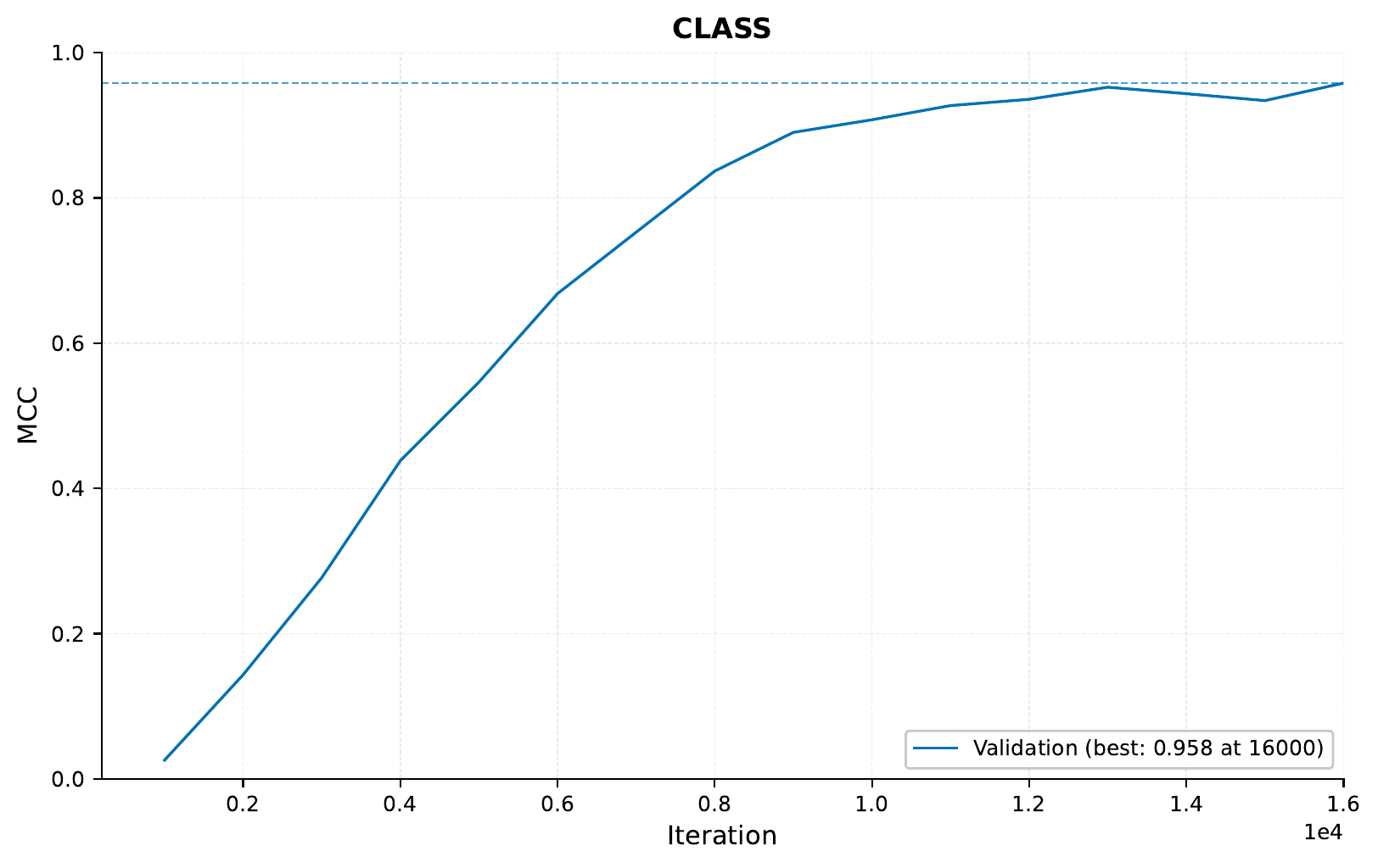
Both look fairly good, but how are we really doing? Let’s check the confusion matrix for our predictions at iteration 15000:

So there it is – we are performing quite well for classes 0-3, but (perhaps as expected), we perform very poorly on the rare classes.
In any case, let’s have a look at how well we do on the test set!
C - Predicting on test set
To test, we can run the following command
(note that you will have to add the path to your saved model for the --model_path
parameter below).
eirpredict \
--global_configs eir_tutorials/a_using_eir/02_tabular_tutorial/conf/02_poker_hands_globals.yaml \
--input_configs eir_tutorials/a_using_eir/02_tabular_tutorial/conf/02_poker_hands_input_test.yaml \
--fusion_configs eir_tutorials/a_using_eir/02_tabular_tutorial/conf/02_poker_hands_fusion.yaml \
--output_configs eir_tutorials/a_using_eir/02_tabular_tutorial/conf/02_poker_hands_output_test.yaml \
--model_path eir_tutorials/tutorial_runs/a_using_eir/tutorial_02_run/saved_models/tutorial_02_run_checkpoint_16000_perf-average=0.8047.pt \
--evaluate \
--output_folder eir_tutorials/tutorial_runs/a_using_eir/tutorial_02_run/
This will create the following extra files
in the eir_tutorials/tutorial_runs/a_using_eir/tutorial_02_run
directory
├── CLASS
│     ├── confusion_matrix.png
│     ├── mc_pr_curve.png
│     ├── mc_roc_curve.png
│     └── predictions.csv
├── calculated_metrics.json
The calculated_metrics.json file
can be quite useful,
as it contains the performance of
our model on the test set.
{"poker_prediction": {"CLASS": {"poker_prediction_CLASS_mcc": 0.9644508846364627, "poker_prediction_CLASS_acc": 0.9799319799319799, "poker_prediction_CLASS_roc-auc-macro": 0.9171988547648481, "poker_prediction_CLASS_ap-macro": 0.4738984488054876, "poker_prediction_CLASS_loss": 0.09111889451742172}}, "average": {"average": {"loss-average": 0.09111889451742172, "perf-average": 0.7851827294022661}}}
This seems pretty good, but we don’t really have any baseline to compare it to. Luckily, there is an great paper titled TabNet: Attentive Interpretable Tabular Learning, which is also using NNs on tabular data, and they even use the Poker Hand dataset as well!
Model |
Test accuracy (%) |
|---|---|
DT |
50.0 |
MLP |
50.0 |
Deep neural DT |
65.1 |
XGBoost |
71.1 |
LightGBM |
70.0 |
CatBoost |
66.6 |
TabNet |
99.2 |
Rule-based |
100.0 |
So using our humble model before we saw an accuracy of around 99%. Of course, since the dataset is highly imbalanced, it can be difficult to compare with the numbers in the table above. For example it can be that TabNet is performing very well on the rare classes, which will not have a large effect on the total test accuracy. However, our performance is perhaps a nice baseline, especially since TabNet is a much more complex model, and we did not do extensive hyper-parameter tuning!
E - Serving
In this final section, we demonstrate serving our trained model as a web service and interacting with it using HTTP requests.
Starting the Web Service
To serve the model, use the following command:
eirserve --model-path [MODEL_PATH]
Replace [MODEL_PATH] with the actual path to your trained model. This command initiates a web service that listens for incoming requests.
Here is an example of the command:
eirserve \
--model-path eir_tutorials/tutorial_runs/a_using_eir/tutorial_02_run/saved_models/tutorial_02_run_checkpoint_16000_perf-average=0.8047.pt
Sending Requests
With the server running, we can now send requests. For tabular data, we send the payload directly as a Python dictionary.
Here’s an example Python function demonstrating this process:
import requests


def send_request(url: str, payload: list[dict]):
    response = requests.post(url, json=payload)
    return response.json()


payload = [
    {
        "poker_hands": {
            "S1": "3",
            "C1": "12",
            "S2": "3",
            "C2": "2",
            "S3": "3",
            "C3": "11",
            "S4": "4",
            "C4": "5",
            "S5": "2",
            "C5": "5",
        }
    }
]

response = send_request(url="http://localhost:8000/predict", payload=payload)
print(response)
When running this, we get the following output:
{
    "result": [
        {
            "poker_prediction": {
                "CLASS": {
                    "0": 3.8413454639396605e-09,
                    "1": 0.9999964237213135,
                    "2": 2.8942279186594533e-06,
                    "3": 6.304654220912198e-07,
                    "4": 5.131337195429797e-12,
                    "5": 1.3689251510129452e-08,
                    "6": 1.3278343702349815e-10,
                    "7": 2.5099328865296755e-11,
                    "8": 2.2613148686900786e-08,
                    "9": 8.275274215874262e-11
                }
            }
        }
    ]
}
We can also send the same request using the curl command:
curl -X POST \
        "http://localhost:8000/predict" \
        -H "accept: application/json" \
        -H "Content-Type: application/json" \
        -d '[{"poker_hands": {"S1": "3", "C1": "12", "S2": "3", "C2": "2", "S3": "3",
         "C3": "11", "S4": "4", "C4": "5", "S5": "2", "C5": "5"}}]'
When running this, we get the following output:
{
    "result": [
        {
            "poker_prediction": {
                "CLASS": {
                    "0": 3.8413454639396605e-09,
                    "1": 0.9999964237213135,
                    "2": 2.8942279186594533e-06,
                    "3": 6.304654220912198e-07,
                    "4": 5.131337195429797e-12,
                    "5": 1.3689251510129452e-08,
                    "6": 1.3278343702349815e-10,
                    "7": 2.5099328865296755e-11,
                    "8": 2.2613148686900786e-08,
                    "9": 8.275274215874262e-11
                }
            }
        }
    ]
}
Analyzing Responses
After sending requests to the served model, the responses can be analyzed. These responses provide insights into the model’s predictions based on the input data.
[
    {
        "request": [
            {
                "poker_hands": {
                    "S1": "3",
                    "C1": "12",
                    "S2": "3",
                    "C2": "2",
                    "S3": "3",
                    "C3": "11",
                    "S4": "4",
                    "C4": "5",
                    "S5": "2",
                    "C5": "5"
                }
            }
        ],
        "response": {
            "result": [
                {
                    "poker_prediction": {
                        "CLASS": {
                            "0": 3.8413454639396605e-09,
                            "1": 0.9999964237213135,
                            "2": 2.8942279186594533e-06,
                            "3": 6.304654220912198e-07,
                            "4": 5.131337195429797e-12,
                            "5": 1.3689251510129452e-08,
                            "6": 1.3278343702349815e-10,
                            "7": 2.5099328865296755e-11,
                            "8": 2.2613148686900786e-08,
                            "9": 8.275274215874262e-11
                        }
                    }
                }
            ]
        }
    }
]
If you made it this far, I want to thank you for reading. I hope this tutorial was useful / interesting to you!